In Part 1, we worked through the theory — embeddings, cosine similarity, and why a dedicated database is needed once you’re dealing with more than a handful of documents. That article ended with toy 3-dimensional vectors we hand-scored ourselves. This one is entirely hands-on. By the end of it, you’ll have a real semantic search tool running on your machine, over your own text, using an actual embedding model instead of numbers we made up.

Background: why Chroma to start with

There are several solid vector databases out there, and we’ll compare them properly in Part 4 once you understand what you’re actually comparing. For this article, we’re starting with Chroma, for one practical reason: it needs no infrastructure. No Docker container to run, no cloud account to sign up for, no API key to manage before you’ve even seen it work. pip install chromadb gets you a fully functional vector database that runs in-process or persists to a local folder on disk. That makes it the fastest path to understanding the mechanics by actually using them, which is the point of this part of the series.

Setting up

You’ll need Python 3.9 or later. Create a virtual environment and install the one package we need:

python3 -m venv venv
source venv/bin/activate        # on Windows: venv\Scripts\activate
pip install chromadb

That’s it for setup. Chroma ships with a default embedding model built in — a small, fast sentence-transformer model called all-MiniLM-L6-v2 — so you don’t need a separate embedding API or key just to follow along. We’ll swap in a stronger, hosted embedding model later in this article once the fundamentals are working.

Your first collection

In Chroma, a collection is roughly the vector-database equivalent of a table in a relational database — a named group of vectors, along with the documents and metadata they came from.

import chromadb
# In-memory client — data disappears when the process exits.
# Good for experimenting; we'll switch to persistent storage shortly.
client = chromadb.Client()
collection = client.create_collection(name="notes")

Now let’s add some documents. Since we haven’t specified an embedding function, Chroma uses its default one automatically — you don’t need to call an embedding model yourself for this to work:

collection.add(
    documents=[
        "The Eiffel Tower is located in Paris, France.",
        "Python is a popular programming language for data science.",
        "The Great Wall of China is visible from low Earth orbit under ideal conditions.",
        "Neural networks are inspired by the structure of the human brain.",
        "Paris is also known for the Louvre, one of the world's largest art museums.",
    ],
    ids=["doc1", "doc2", "doc3", "doc4", "doc5"],
)

Every document needs a unique id. Think of it as a primary key — Chroma uses it internally to know what to update if you re-add the same document later.

Running a query

Now let’s ask a question in plain English and see whether Chroma returns the right documents even when the wording doesn’t match:

results = collection.query(
    query_texts=["What famous landmarks are in the French capital?"],
    n_results=2,
)
for doc, distance in zip(results["documents"][0], results["distances"][0]):
    print(f"{distance:.4f}  {doc}")

This should print something close to:

0.62  The Eiffel Tower is located in Paris, France.
0.81  Paris is also known for the Louvre, one of the world's largest art museums.

The exact numbers will vary slightly depending on your Chroma and embedding model versions, but the ranking should hold. Notice that the query never said “Eiffel Tower,” “Paris,” or “Louvre” — it said “landmarks” and “French capital.” Chroma found the right documents because the embedding model understood what those phrases mean. This is the same idea from Part 1, except now it’s running as real code against a real embedding model, not a hand-crafted example.

One detail worth flagging so it doesn’t trip you up later: Chroma’s default metric returns a distance, not a similarity score, so lower is better here — the opposite of the cosine similarity numbers from Part 1, where higher meant more similar.

Making it persistent

The in-memory client above throws away everything the moment your script ends, which is fine for experimenting but not much else. For anything real, use a PersistentClient, which writes to disk:

import chromadb
client = chromadb.PersistentClient(path="./chroma_store")
collection = client.get_or_create_collection(name="notes")

In practice, you’ll want get_or_create_collection rather than create_collection most of the time — it won’t throw an error if the collection already exists from a previous run, which is exactly the situation you’re in every time you restart a script that’s meant to reuse an existing index.

Adding metadata and filtering on it

Real documents come with context — a source, a date, a category — and Chroma lets you attach arbitrary metadata to each document, then filter on it at query time. This is what lets you combine semantic similarity with the kind of exact filtering you’d expect from a traditional database, rather than choosing one or the other:

collection.add(
    documents=[
        "Quarterly revenue grew 12% year over year.",
        "The new hiking trail opens to the public in June.",
        "Cloud infrastructure costs were reduced by 20% this quarter.",
    ],
    ids=["fin1", "outdoor1", "fin2"],
    metadatas=[
        {"category": "finance", "year": 2026},
        {"category": "lifestyle", "year": 2026},
        {"category": "finance", "year": 2026},
    ],
)
# Semantic search, restricted to the "finance" category only
results = collection.query(
    query_texts=["How did costs change?"],
    n_results=5,
    where={"category": "finance"},
)
print(results["documents"][0])

This where filter is what makes vector databases practical for real applications. You almost never want to search your entire dataset — you want to search “my documents,” or “documents from this quarter,” or “public content only” — and being able to express that in the same query as the semantic search is what separates a toy demo from something you’d actually deploy.

Putting it together: a working search tool over your own notes

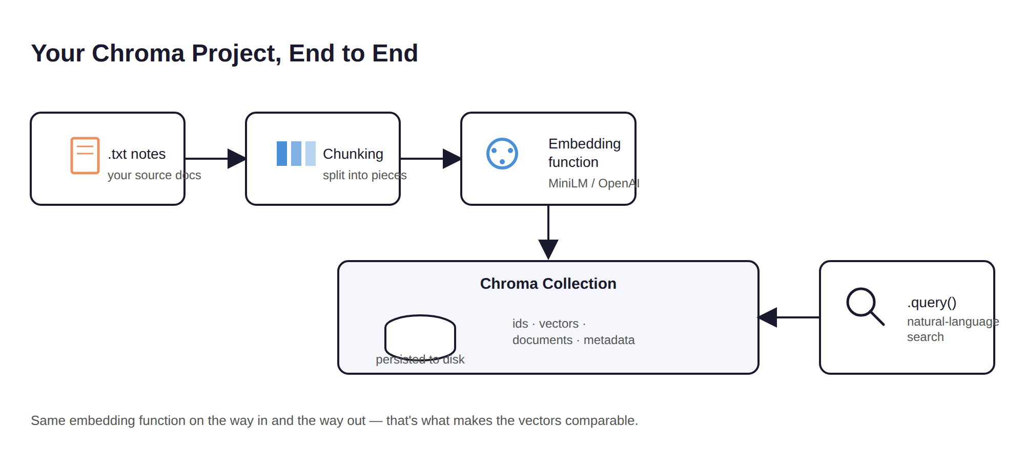
Let’s build something you can actually use — a small command-line tool that indexes a folder of .txt files and lets you search them semantically.

import os
import sys
import chromadb
def build_index(notes_dir: str, db_path: str = "./notes_db"):
    client = chromadb.PersistentClient(path=db_path)
    collection = client.get_or_create_collection(name="my_notes")
    documents, ids, metadatas = [], [], []
    for filename in os.listdir(notes_dir):
        if not filename.endswith(".txt"):
            continue
        filepath = os.path.join(notes_dir, filename)
        with open(filepath, "r", encoding="utf-8") as f:
            content = f.read().strip()
        if content:
            documents.append(content)
            ids.append(filename)
            metadatas.append({"filename": filename})
    if documents:
        # upsert avoids duplicate-id errors if you re-index the same files
        collection.upsert(documents=documents, ids=ids, metadatas=metadatas)
    print(f"Indexed {len(documents)} notes into '{db_path}'")
    return collection
def search(collection, query: str, n_results: int = 3):
    results = collection.query(query_texts=[query], n_results=n_results)
    for doc, meta, dist in zip(
        results["documents"][0], results["metadatas"][0], results["distances"][0]
    ):
        print(f"\n[{meta['filename']}]  (distance: {dist:.4f})")
        print(doc[:200] + ("..." if len(doc) > 200 else ""))
if __name__ == "__main__":
    notes_dir = sys.argv[1] if len(sys.argv) > 1 else "./notes"
    client = chromadb.PersistentClient(path="./notes_db")
    collection = client.get_or_create_collection(name="my_notes")
    if len(sys.argv) > 2 and sys.argv[2] == "--index":
        build_index(notes_dir)
    else:
        query = input("Search your notes: ")
        search(collection, query)

To try it out:

mkdir notes
echo "Meeting notes: we decided to delay the launch to Q3 for more QA time." > notes/meeting1.txt
echo "Grocery list: eggs, spinach, olive oil, oat milk." > notes/groceries.txt
echo "Project retro: the launch delay gave us time to fix three critical bugs." > notes/retro.txt
python search_notes.py ./notes --index
python search_notes.py ./notes
# Search your notes: why did we push the release date back?

Try that exact query — “why did we push the release date back?” — against notes that never use the words “push,” “release,” or “back.” If retrieval is working as expected, meeting1.txt and retro.txt should come back ahead of groceries.txt, because the model understands “delay the launch” and “push the release date back” as the same idea, even though not one word matches literally.

Swapping in a stronger embedding model

The default embedding model is fast and needs no API key, which is exactly what you want while you’re learning. For production quality, though, most teams reach for a stronger hosted model — OpenAI’s text-embedding-3-large is a common choice. Chroma makes this a one-line change through an embedding function:

from chromadb.utils import embedding_functions
openai_ef = embedding_functions.OpenAIEmbeddingFunction(
    api_key="YOUR_OPENAI_API_KEY",
    model_name="text-embedding-3-large",
)
collection = client.get_or_create_collection(
    name="my_notes_openai",
    embedding_function=openai_ef,
)

Everything else — .add(), .query(), .upsert() — stays exactly the same. This is one of the genuinely useful properties of how vector databases are designed: the storage and search layer is decoupled from the embedding model itself, so upgrading embedding quality later doesn’t mean rewriting your application logic. It does mean re-embedding and re-indexing your existing documents, though, since vectors from two different models are never directly comparable — worth keeping in mind before you switch models on a large, already-indexed dataset.

What you’ve built

At this point you have a genuinely working semantic search tool. It indexes arbitrary text, embeds it with a real model, persists the index to disk, and answers natural-language queries by meaning rather than keyword — with metadata filtering available when you need it. That’s already useful on its own, for something like searching personal notes, support tickets, or a small document archive.

What’s next

Semantic search retrieves relevant text, but it doesn’t answer a question — it just tells you where the answer probably is. In Part 3, we take this exact index and connect it to a large language model to build a full RAG (Retrieval-Augmented Generation) pipeline: the retrieved documents become context the LLM uses to generate a grounded answer, with citations back to the original notes.

Series roadmap:

• Part 1: Fundamentals — embeddings, similarity, how vector search works
• Part 2 (this article): Hands-on — build a working semantic search tool with Chroma
• Part 3: Build a full RAG Q&A pipeline over your own documents
• Part 4: Production, scaling, indexing internals, and hybrid vector + graph systems