

I started digging into vector databases the way most engineers probably do — I kept running into the term “RAG” in conversations about AI systems, and every explanation I found assumed I already knew what a vector database was, how similarity search worked, and why you’d need one in the first place. So I went back to basics and worked it out properly, and this series is the result.
This is Part 1 of a four-part series. In this article we will build the conceptual foundation — what an embedding actually is, how “similarity” gets measured mathematically, and why a specialized database is needed at all instead of just looping over your data. Part 2 gets hands-on and installs a real vector database on your machine. Part 3 turns that into a working RAG pipeline. Part 4 covers what changes when you take this to production. If you are comfortable with basic Python and have never worked with embeddings before, this article is written for you.
Background: the problem we’re actually solving
Traditional databases are built to answer exact questions. SELECT * FROM products WHERE category = 'shoes' works well when you know precisely what you’re looking for, because the database is matching values exactly.
But that’s not how people actually search. Someone types “affordable running shoes for flat feet,” and a keyword-based system will miss a product titled “budget-friendly sneakers with arch support” — even though it’s exactly what the person wants — simply because the words don’t overlap. The gap here isn’t a bug in the search engine. It’s that keyword matching compares words, while the user is actually expressing meaning.
Vector databases exist to close that gap. They do this by converting text (or images, or audio) into embeddings — lists of numbers that represent meaning in a way a computer can compare mathematically. Two pieces of content that mean similar things end up with similar numbers, regardless of whether they share a single word.
Understanding the concept: what is an embedding, really?
Let us try to understand this with a simplified example before we bring in any real embedding model.
Imagine we only cared about three properties of a sentence: how much it’s about animals, how much it’s about food, and how much it’s about technology. We could hand-score a few sentences on those three axes:
| Sentence | animal-ness | food-ness | tech-ness |
|---|---|---|---|
| “The cat sat on the mat” | 0.90 | 0.10 | 0.00 |
| “Dogs are loyal animals” | 0.95 | 0.00 | 0.00 |
| “Python is a programming language” | 0.10 | 0.00 | 0.90 |
| “I love eating pizza” | 0.00 | 0.90 | 0.00 |
| “Machine learning uses neural networks” | 0.00 | 0.00 | 0.95 |
Each row is a 3-dimensional embedding. This is exactly what a real embedding model does, except it isn’t hand-scored — it’s learned automatically from patterns in the text it was trained on, and instead of three human-readable dimensions like “animal-ness,” a real model typically uses somewhere between 384 and 1536 dimensions that don’t map to anything a human would label directly. The idea is the same. Only the scale and the interpretability change.
Why do we need a way to measure “closeness”?
Once content is represented as vectors, “how similar are these two things” stops being a language question and becomes a geometry question — how close together do their vectors point? The most common way to measure this is cosine similarity. It looks at the angle between two vectors rather than their raw distance, which is what makes it robust to differences in text length — a one-line summary and a three-paragraph explanation of the same idea can still score as highly similar.
Let’s prove this with the toy embeddings from the table above, instead of just taking the claim on faith. Say a user searches “Tell me about pets,” which we’ll hand-embed as [0.85, 0.05, 0.00] — heavily animal-leaning, barely food-leaning, not tech at all:
import numpy as np# Toy embeddings: each vector is [animal-ness, food-ness, tech-ness]# A real embedding model learns dimensions like this automatically,# just with hundreds of dimensions instead of three human-readable ones.docs = { "The cat sat on the mat": [0.90, 0.10, 0.00], "Dogs are loyal animals": [0.95, 0.00, 0.00], "Python is a programming language": [0.10, 0.00, 0.90], "I love eating pizza": [0.00, 0.90, 0.00], "Machine learning uses neural networks": [0.00, 0.00, 0.95],}def cosine_similarity(a, b): a, b = np.array(a), np.array(b) denom = np.linalg.norm(a) * np.linalg.norm(b) return float(np.dot(a, b) / denom) if denom > 0 else 0.0query_vec = [0.85, 0.05, 0.00] # "Tell me about pets"results = sorted(docs.items(), key=lambda kv: -cosine_similarity(query_vec, kv[1]))for doc, vec in results: print(f"{cosine_similarity(query_vec, vec):.3f} {doc}")
Running this gives:
0.999 The cat sat on the mat0.998 Dogs are loyal animals0.110 Python is a programming language0.059 I love eating pizza0.000 Machine learning uses neural networks
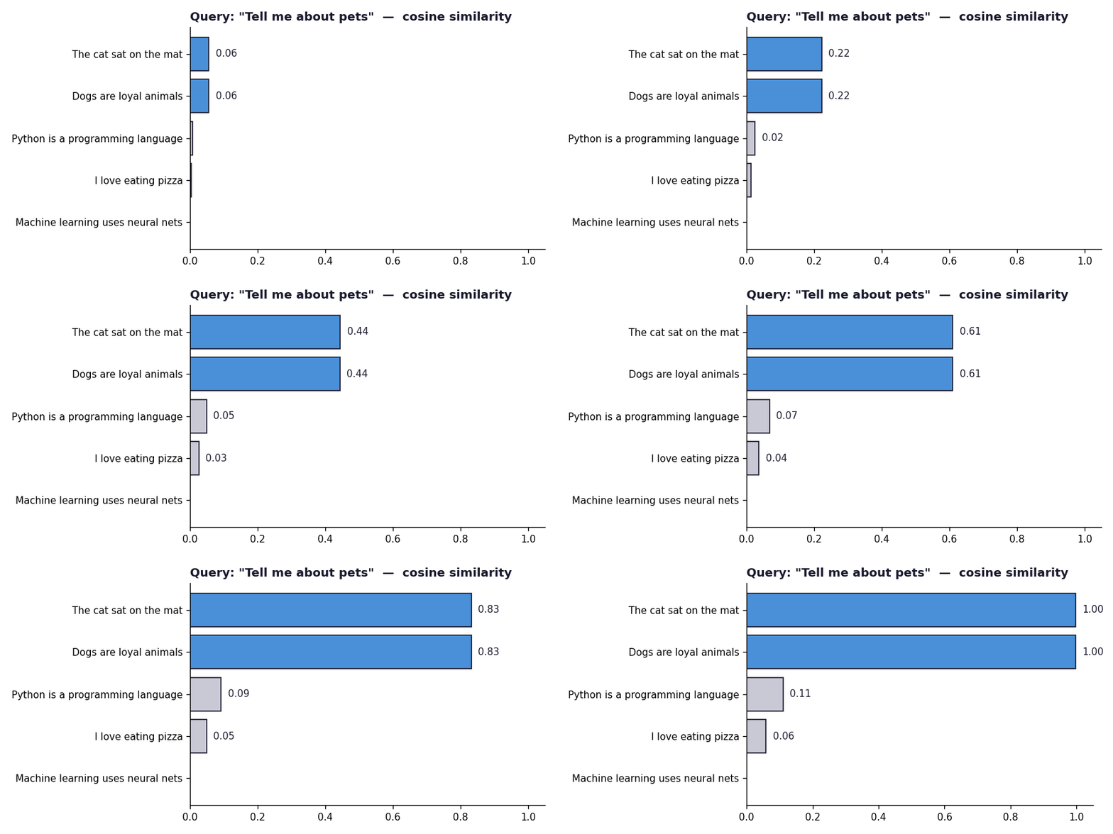
Notice what just happened here. The query never contained the words “cat,” “dog,” or “mat.” It surfaced the right documents anyway, purely because their meaning was close to the query’s meaning in vector space. That, in one small worked example, is the entire premise behind semantic search.
So what does a vector database actually add?
The code above is, technically, a complete (if tiny) vector search system — and it’s worth pausing on what it’s actually doing under the hood, because that operation is the core of every vector database: given a query vector, find the k stored vectors that are most similar to it. This is called k-nearest-neighbors (k-NN) search.
Now the question arises — if five lines of Python can already do this, why do we need a dedicated database at all?
The answer is scale. Comparing a query against five documents is instant, on any hardware. Comparing it against fifty million documents, using the same brute-force loop, is not — that’s fifty million similarity calculations for every single query. A vector database exists specifically to make this fast at scale, and it does three things a plain Python loop does not:
- Indexing. Instead of comparing against every stored vector, a vector database builds a data structure — commonly HNSW, short for Hierarchical Navigable Small World graphs — that lets it find approximate nearest neighbors in roughly logarithmic time instead of linear time. This is called Approximate Nearest Neighbor (ANN) search, and it trades a small amount of accuracy for a large amount of speed. We’ll go into how HNSW actually works in Part 4, once we have a real system to reason about.
- Storage and persistence. It stores vectors alongside metadata — the original text, tags, timestamps, permissions — and persists all of it to disk, so you aren’t re-embedding your entire dataset every time a process restarts.
- Filtering and hybrid queries. In practice you rarely want to search your entire dataset. You want “find similar items, but only from category X” or “only from documents added in the last 30 days.” A vector database lets you combine vector similarity with ordinary metadata filters in a single query, which a plain in-memory loop doesn’t give you for free.
How search works end to end
Here is the full pipeline, drawn out:
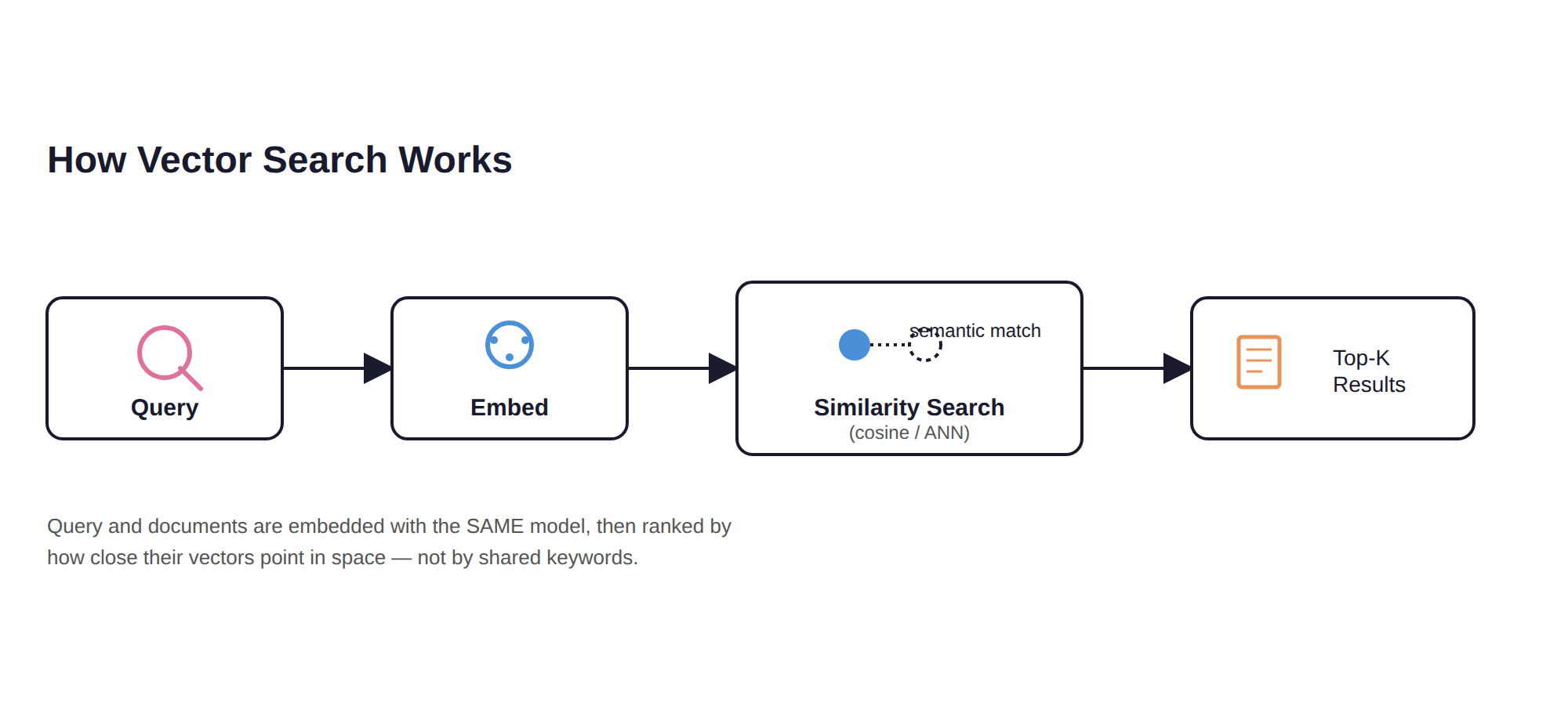
- Query — the user’s raw text, image, or audio input.
- Embed — the same embedding model used to embed your documents converts the query into a vector. This consistency matters more than it might seem: you cannot mix embeddings from two different models and expect meaningful comparisons, because different models place meaning in different vector spaces. A vector from OpenAI’s embedding model and a vector from an open-source model are not directly comparable, even if both represent the same sentence.
- Similarity search — the vector database’s index finds the vectors closest to the query vector.
- Top-K results — the k most similar items come back, typically ranked by similarity score.
Practical considerations: where vector databases shine, and where they don’t
Vector databases are a strong fit for semantic search and question answering, document and knowledge-base retrieval — including as the retrieval half of RAG, which we’ll build in Part 3 — recommendation systems, and image or audio similarity search. They’re fast at scale, and they don’t require you to explicitly model relationships between items, because the embedding model captures that implicitly.
That last point is also their limitation. Vector databases have limited native support for explicit relationships and structure. If your problem is fundamentally about multi-hop reasoning — “find the suppliers of the supplier of this company that operates in a sanctioned region” — a vector database alone will struggle, because there’s no explicit notion of “supplier of” in a similarity score. That kind of query is a much better fit for a graph database, which models entities and relationships directly and is built for traversal.
This isn’t really a competition between the two. Production systems increasingly combine them — vector search for “what’s semantically relevant,” graph traversal for “how is this connected to that.” We’ll cover that hybrid approach properly in Part 4.
A quick note on the landscape
You don’t need to memorize any of this, but it helps to know the landscape before Part 2, where we’ll pick a starting point.
For embedding models, commonly used options today include OpenAI’s text-embedding-3-large, Cohere’s Embed v3, and strong open-source alternatives like BAAI’s BGE-M3 and intfloat’s E5-large. The open-source models run locally at no API cost, at some tradeoff in quality against the strongest hosted models.
For vector stores, the range goes from developer-friendly and easy to run locally — Chroma is the clearest example — through production-oriented open-source systems like Qdrant, Milvus, and Weaviate, up to fully managed cloud services like Pinecone. PostgreSQL with the pgvector extension is also widely used when a team wants vector search inside a database they already operate, rather than adding a new system.
What we’ve covered, and what’s next
We’ve established what an embedding is, why cosine similarity gives us a mathematical notion of “meaning is close,” and why a dedicated database — not a Python loop — is what makes this practical at real scale. In Part 2, we get hands-on: install a real vector database, Chroma, on your machine, embed a small set of actual documents with a real embedding model, and run real semantic search queries — no toy vectors this time. By the end of Part 2, you’ll have a working semantic search tool over your own text.
Series roadmap:
- Part 1 (this article): Fundamentals — embeddings, similarity, how vector search works
- Part 2: Hands-on — build a working semantic search tool with Chroma
- Part 3: Build a full RAG Q&A pipeline over your own documents
- Part 4: Production, scaling, indexing internals, and hybrid vector + graph systems


