
Parts 1 through 3 took us from “what is an embedding” to a working RAG pipeline running locally on Chroma. Everything worked, but everything also ran on a laptop, against a few dozen text files. This final article covers what actually changes once that same pipeline needs to serve real users against a real dataset — and it closes with the hybrid vector-plus-graph architecture that production RAG systems increasingly reach for.
Background: what “approximate” nearest neighbor actually means
In Part 1, we mentioned that vector databases use Approximate Nearest Neighbor (ANN) search instead of brute-force comparison, trading a small amount of accuracy for a large amount of speed. It’s worth understanding why that tradeoff exists before we talk about tuning it.
Brute-force k-NN search is exact — it compares your query vector against every stored vector and returns the true top-k closest matches. The problem is that it’s O(n) per query: search time grows linearly with the number of vectors. At ten thousand vectors, this is instant. At a hundred million vectors, even fast hardware takes a noticeable amount of time per query, and that cost is paid on every single search, not just the first one.
HNSW, short for Hierarchical Navigable Small World, is the indexing algorithm behind most modern vector databases — Chroma, Qdrant, Weaviate, and Milvus all use some variant of it. It solves the scaling problem by building a multi-layer graph structure at insert time:
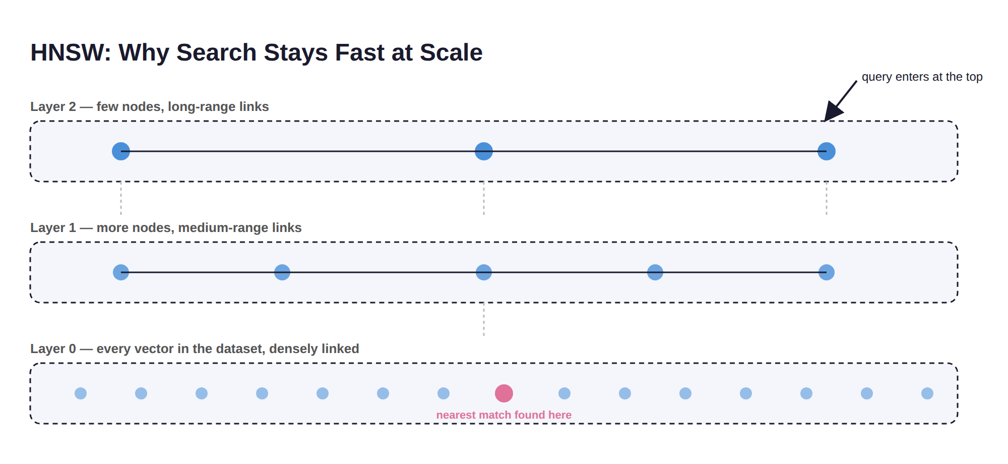
- The top layer contains a sparse set of long-range links between distant points, letting a search jump across the vector space quickly.
- Lower layers get progressively denser, with more local connections between nearby points.
- A query starts at the top layer, greedily navigates toward the query vector, then drops down a layer and repeats — narrowing in on the true nearest neighbors without ever touching most of the dataset.
This gets you roughly O(log n) search time instead of O(n), which is the difference between a search that stays fast at a hundred million vectors and one that doesn’t. The cost is twofold: the search is now approximate, meaning it can occasionally miss the true nearest neighbor in favor of one that’s very close, and building the index takes memory and insert-time compute — which is why bulk-loading a vector database is usually noticeably faster than inserting vectors one at a time.
Two parameters show up in every major vector database’s HNSW configuration, and they’re worth knowing by name:
ef_constructioncontrols how thorough the search is while building the index. Higher values produce a better-quality graph, at the cost of slower indexing.ef_search(sometimes justef) controls how thorough the search is at query time. Higher values improve recall — you’re less likely to miss a true nearest neighbor — at the cost of query latency.
These two are the main levers for trading off speed, accuracy, and memory in a production vector database. If search feels either too slow or subtly low-quality, this is usually the first place to look.
Choosing a vector database for production
Part 2 used Chroma because it needs no setup at all. In production, the right choice depends on your actual constraints, not on which one is trending:
| Database | Good fit when… |
|---|---|
| Chroma | Prototyping, small-to-medium datasets, embedded or local deployment, simplicity matters more than massive scale |
| Qdrant | You want a fast, production-grade open-source option with strong filtering, self-hosted via Docker or their managed cloud |
| Weaviate | You want built-in hybrid (keyword + vector) search and a GraphQL-style API out of the box |
| Milvus | You’re operating at very large scale — billions of vectors — and need a distributed, horizontally scalable system |
| Pinecone | You want a fully managed service with no infrastructure to operate, and you’re fine with a cloud dependency and its pricing model |
| PostgreSQL + pgvector | You already run Postgres and want vector search alongside your existing relational data, without adding a new system to operate |
A practical rule of thumb: start with whatever has the least operational overhead for your team — often Chroma, or pgvector if you already run Postgres — and only migrate to a dedicated, horizontally scalable system like Qdrant or Milvus once load testing or real traffic gives you evidence that you actually need it. Migrating early, before you have that evidence, mostly adds operational burden you may never end up needing to pay for.
Improving retrieval quality: hybrid search and reranking
Pure vector search has a specific weakness. It’s excellent at semantic matching, but it can miss exact matches — product SKUs, error codes, proper nouns, acronyms — because embedding models compress meaning in ways that sometimes blur precise tokens. Hybrid search addresses this by combining vector similarity with traditional keyword search, commonly BM25, and merging the two ranked lists. That gives you semantic recall and exact-match precision together, rather than having to pick one. Weaviate and Qdrant both support this natively; with Chroma or a custom setup, you’d typically run a keyword search — through Postgres full-text search or Elasticsearch, for example — alongside the vector query and merge the results yourself.
Reranking, mentioned briefly in Part 3, is the other major lever. The pattern is: retrieve a larger candidate set — say, the top 20 — using a cheap, fast method like vector search, then pass those 20 candidates through a slower but more precise reranking model, a cross-encoder that scores query-document pairs directly rather than comparing pre-computed vectors, to select the final top 3 to 5 that actually go into the LLM’s context. This two-stage “retrieve, then rerank” pattern consistently outperforms single-stage vector search alone in production RAG evaluations, because a cross-encoder can model the query and document jointly instead of compressing each one independently into a fixed vector ahead of time.
When to reach for a graph database instead — or alongside
The infographic that started this series drew a clear line between vector and graph databases, and it’s worth restating precisely, because this is the most common architecture decision teams face in this space:
| Feature | Vector DB | Graph DB | Hybrid (GraphRAG) |
|---|---|---|---|
| Semantic search | Strong | Moderate | Strong |
| Explicit relationships | Weak | Strong | Strong |
| Multi-hop reasoning | Weak | Strong | Strong |
| Scale & speed | Fast | Moderate | Fast / balanced |
| Context richness | Moderate | Strong | Very strong |
A graph database — Neo4j, Amazon Neptune, ArangoDB, TigerGraph, Memgraph — models data as explicit nodes and relationships: LangChain --is_a--> Python Library, RAG --requires--> Vector DB. It excels at queries that require traversal — what connects to what, how many hops away, and through which path. That’s the natural fit for fraud detection, compliance and audit trails, org-chart or supply-chain analysis, and generally any question shaped like “how is X related to Y” rather than “what is semantically similar to X.”
The two aren’t competing approaches, and combining them — often called GraphRAG — is increasingly the architecture of choice for RAG systems that need to answer genuinely complex, multi-hop questions that a pure vector search would miss.
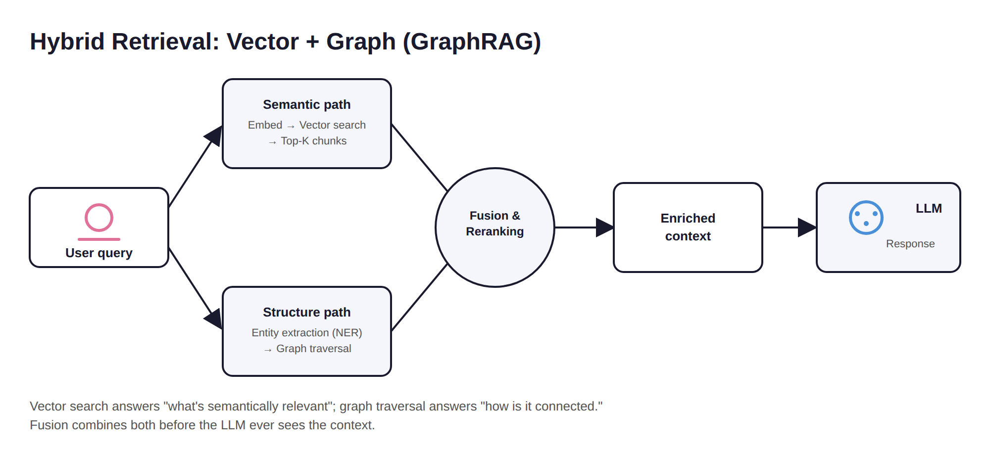
In practice, this means running your normal vector retrieval from Part 3, and, in parallel, extracting named entities from the query and traversing a knowledge graph to find related entities and structured facts, then merging and reranking both result sets before handing the combined context to the LLM. Common production pairings include Neo4j with Pinecone, Neo4j with Qdrant, and Amazon Neptune with Qdrant; ArangoDB offers native hybrid support inside a single system. Frameworks like LangChain, LlamaIndex, and dedicated GraphRAG pipelines provide scaffolding for orchestrating this, so you’re not hand-rolling the fusion logic from scratch.
Worth being direct about when to actually reach for this: don’t build a hybrid system by default. It roughly doubles your infrastructure and pipeline complexity. Reach for it specifically when your evaluation shows your RAG system consistently fails on questions that require connecting multiple pieces of structured information — dates, ownership, hierarchy, causality — that a document chunk alone can’t answer. As a simple decision rule, echoing the original infographic: pure semantic QA or similarity search means a vector database is fine; relationship-heavy or multi-hop queries mean it’s worth considering a graph database; complex multi-hop questions on top of semantic RAG mean hybrid GraphRAG is worth considering.
Operating a vector database in production
A few practical concerns that don’t show up in tutorials, but matter once real traffic hits your system:
Re-embedding on model upgrades. If you switch embedding models — even to a newer version of the same model family — every existing vector becomes incomparable to new queries, because different models place meaning in different vector spaces, as we covered in Part 1. That means a full re-index of your entire corpus. Budget for this as a recurring maintenance cost, not a one-time setup step you do once and forget.
Freshness. Documents change. Decide upfront whether your index needs near-real-time updates — a support ticket system, where stale answers are actively harmful — or can tolerate batch re-indexing on a schedule, like a mostly-static product catalog. This decision drives your update strategy: streaming upserts versus periodic full rebuilds.
Monitoring retrieval quality, not just uptime. A vector database can look perfectly healthy from an infrastructure standpoint — low latency, no errors — while silently returning poor results because of a chunking regression or a metadata filter bug. Track retrieval-specific metrics, such as recall against a labeled evaluation set of query-and-expected-document pairs, the same way you’d track model accuracy, not just service uptime.
Cost at scale. Embedding is billed per token on hosted APIs, and it’s easy to underestimate the cost of re-embedding large corpora repeatedly during development. Vector storage itself has a real memory footprint too — HNSW indexes are typically held in RAM for query speed, so a hundred-million-vector index at 1536 dimensions can require substantial memory before you’ve even accounted for metadata.
Closing the series
Across four parts, we went from a static infographic to understanding what an embedding is and why cosine similarity works, to building a real semantic search tool with Chroma, to extending it into a full RAG pipeline with grounded, cited answers, to understanding what changes — indexing internals, hybrid search, reranking, and graph-augmented retrieval — when that system needs to run in production at scale.
The honest summary of when to use what:
If you need fast semantic search or question answering over unstructured content, a vector database alone, as built in Parts 2 and 3, is usually enough. If you need to reason over explicit relationships — who’s connected to whom, through how many hops — add a graph database. If you need both, in a system that has to answer genuinely complex questions, a hybrid GraphRAG architecture is worth considering — but only once evaluation evidence tells you a pure vector approach is actually falling short, not as a default starting point for a new project.
Series roadmap:
- Part 1: Fundamentals — embeddings, similarity, how vector search works
- Part 2: Hands-on — build a working semantic search tool with Chroma
- Part 3: Build a full RAG Q&A pipeline over your own documents
- Part 4 (this article): Production, scaling, indexing internals, and hybrid vector + graph systems


